STAGE 06 / 06
Remaining energy becomes heat
WHY THIS HAPPENS
Adjust the anode and emitter field ↗
01 / TECHNOLOGICAL GYROTRONS
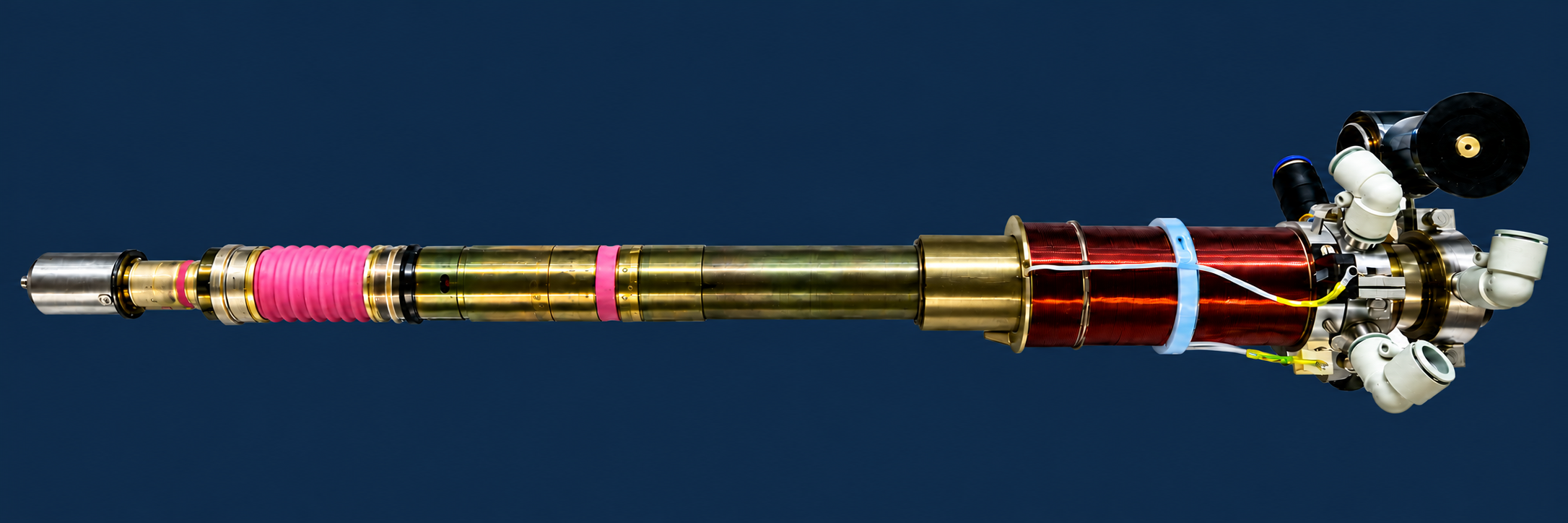
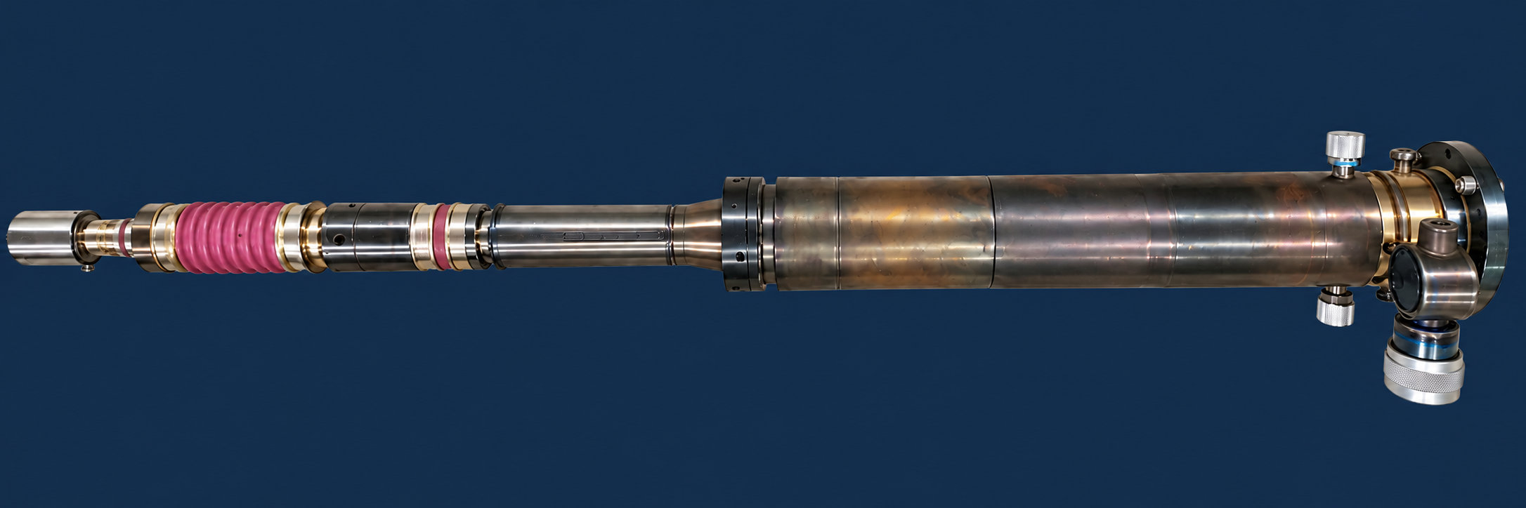
The magnetically shielded system (MSS) generates the main field in the cavity. The field decreases towards the cathode and collector. This version uses a schematic field profile.
Frequency of the selected mode if excited
Relative to the total injected beam power
Magnetic reflection · fraction of Ib
P = η · U₀ · Ib
Intercepted before the cavity
v⊥ / v∥ · transmitted beam
Rc and Zc are taken from INTERACTION PARAMETERS and remain fixed during the search. These dimensions determine the cold-cavity frequency. Only voltages and magnetic fields are varied; Ib is retained.
Numerical search for the best operating point in this teaching model at fixed Rc and Zc. A global efficiency maximum is not guaranteed.
Rc, Zc and frequency are taken from INTERACTION PARAMETERS and held fixed. U₀, Ua, B₀, Bk and Ib ≤ 3 A are selected to maximize P = η·U₀·Ib. This estimates RF power before output-path losses.
Output-path losses, space charge and self-consistent oscillation are not calculated. A global power maximum is not guaranteed.
Phase diagram relative to the RF field, not a transverse beam cross-section.
The light bar is the upper bound at constant p∥, accounting for the transmitted fraction. The colored bar is the calculated energy transfer from the entire injected beam. Energy recovery and output-path losses are excluded.
Stages highlight the part being studied while the full path from the emitter band to the collector remains visible. In steady operation, emission, interaction, RF output and electron collection occur simultaneously.
A nominal frequency of 28 GHz and output power of 10 kW define the reference device. Its operating mode is TE₁,₂ at the first cyclotron harmonic, n = 1. The cavity radius is Rc = 9.05 mm and its uniform section is Zc = 65 mm long. U₀ = 23 kV, anode-to-cathode voltage Ua = 17 kV and beam current Ib = 1 A.
AnGEl report No. 00004196 dated 29.10.2026 gives g = ⟨v⊥⟩/⟨v∥⟩ = 1.6744, transmitted current 1 A and reflected current 0 A. The emitter-center radius is 9 mm and the band is 2 mm long. The emitter center is at z = −157.15 mm; the cavity and main magnetic system are centered at z = 0. B₀ = 1 T and the total emitter-center field is Bk = 0.106 T. Bk is the total field; ΔBk is the cathode-coil contribution. The linear approximation is Bk = 0.106·B₀ + ΔBk, with all fields in T. The coefficient 0.106 is set by the reference point at B₀ = 1 T and ΔBk = 0; separate measured MSS and coil field maps are not provided in the report. MSS saturation, hysteresis and the cathode-coil contribution inside the cavity are not included. Electron-optical system retains its separate teaching reference point.
The scaling p⊥,cavity ∝ Ua√B₀/Bk3/2 is anchored to this reference point. The 100 equal-current particles are calibrated to a mean g = 1.6744 and a full Vp spread of 11.371%. The uniform distribution is an assumption, not a reconstruction of the AnGEl trajectories. Space charge, potential depression and electrode fields are not solved.
The effective g = √(⟨q⟩/(1−⟨q⟩)), with q = p⊥²/p², preserves the mean squared transverse momentum of the transmitted particles for the RF model. At the reference point it is 1.668 ≈ 1.67. The reported compression ratio 9.385 uses more precise internal field values; the rounded ratio 1/0.106 is 9.434. The adiabatic compression model is not applicable when Bk ≤ 0 or E⊥/Bk ≥ c. A local planar crossed-field estimate first classifies electrons intercepted by the anode. Only the remaining electrons are checked for magnetic reflection; g is calculated for the beam transmitted to the cavity.
Anode interception uses the same relativistic Hull criterion as the megawatt laboratory, with an illustrative 8 mm gap and ±8% gap variation. These are teaching assumptions, not AnGEl gun dimensions. Ib = Ipassed + Irf + Ia; the reflected and intercepted currents are excluded from RF injection. Orange trajectories terminate on the anode; normal transmitted electrons remain clear of it. This estimates electron interception, not vacuum-arc inception.
The closed-cylinder equation f₀ = c/(2π)·√[(χ′₁,₂/Rc)² + (π/Zc)²], with χ′₁,₂ = 5.33144277, gives 28.20 GHz. The axial index q = 1 and sinusoidal field profile are teaching assumptions. Open-cavity effects, tapers and frequency pulling are not calculated. At U₀ = 23 kV and B₀ = 1 T, the relativistic cyclotron frequency fc ≈ 26.79 GHz must not be identified with the rounded 28 GHz in the report.
64 initial phases are integrated in a prescribed rotating field at constant p∥. The amplitude, from 0 to 6 MV/m, is selected by the mean energy transfer. P = ηU₀Ib is power transferred to the field, not device output power. The nominal 10 kW corresponds to 43.48% of the 23 kW beam power, but the trajectory report contains no RF calculation or confirmation of this efficiency. Its Wclt = 23 kW is electrical power at the collector without RF interaction. The calculation is not fitted to 10 kW. Losses, self-excitation and mode competition are not calculated.
The high-voltage supply provides energy.
The magnetic field shapes the motion.
The cavity helps transfer energy to the wave.
The Lorentz force changes the velocity direction, but a static magnetic field does no work. Magnetic compression redistributes momentum between axial and transverse motion.
Electrons bunch by their rotation phase relative to the RF field. At suitable settings, the average energy exchange is from beam to wave. Bunching and energy transfer occur within the same cavity.
The electric component of the RF field does work on the electrons, mainly reducing their transverse energy. The cavity field grows and the spent beam enters the collector.
ABOUT THE MODEL
This model describes a technological gyrotron: a magnetron injection gun, MSS, cavity, collector coil and permanent magnets near the axial output window. Component shapes are based on the supplied photographs; dimensions and field maps are set for teaching. The external waveguide is not included.
Equations, selected mode and model limits ↗SOURCES AND FURTHER READING
01 / THEORYElectron cyclotron resonanceSabchevski · Applied Sciences, 2024↗02 / ELECTRON OPTICSMagnetron injection gunZhang, Nix, Cross · IEEE Transactions on Electron Devices, 2020↗03 / DESIGNHigh-power gyrotron developmentGantenbein et al. · Karlsruhe Institute of Technology↗04 / INTERACTIONBunching and energy extractionGyro-device research · MIT Plasma Fusion Center↗МАГНЕТРОННО-ИНЖЕКТОРНАЯ ПУШКА
Нагрейте эмиттер, задайте ускорение и анодное напряжение, настройте поле МЭС и катодную катушку. Проследите путь от эмиссии до отражения и осаждения на коллекторе.
При фиксированных магнитных полях рост Uа–к усиливает поле у эмиттера и в этой модели повышает поперечный импульс. Полная энергия в резонаторе определяется U₀, а формирующее напряжение Uа–к задаёт условия старта. В этой модели ток не влияет на форму траекторий через пространственный заряд.
При фиксированном Bкат рост Bрез повышает p⊥. Здесь МЭС одновременно усиливает свой фон у катода; итоговое изменение α определяется обоими полями, поэтому знак эффекта не универсален.
Сонаправленное добавочное поле повышает Bкат и при остальных фиксированных настройках уменьшает α в выбранной модели. Встречное поле увеличивает α и может вывести часть распределения в отражение.
ПОСЛЕ РЕЗОНАТОРА / КОЛЛЕКТОР
Катушка меняет магнитное поле в коллекторе и положение зоны осаждения. Постоянные магниты у выходного узла помогают осадить остаточные электроны до окна.
Основная зона осаждения показана в средней части коллектора.
Магниты помогают осадить остаточные электроны до окна.
Настройки показывают качественное перемещение зоны, без привязки к току катушки и координатам в мм. Траектории, расположение магнитов и охлаждение схематичны. Для расчёта осаждения и тепловой нагрузки нужны геометрия, карта поля и параметры отработанного пучка.
LaB₆ / ТЕРМОЭМИССИЯ И ОБРАТНАЯ СВЯЗЬ
Нагрев пояска увеличивает термоэмиссию. Если часть возвращающихся электронов попадает на эмиттер и передаёт ему энергию, дополнительный нагрев может усилить эмиссию ещё больше.
Без этого допущения отражённые электроны разворачиваются у электростатического барьера и могут оставаться в ловушке; удар о катод не подразумевается.
Эмиссионный запрос при выбранном Ib: 1,50 А.
Феноменологическая иллюстрация обратной связи. Время и коэффициент нагрева условны; это не прогноз температуры, тока или порога неустойчивости реального гиротрона.
α = v⊥/v∥. Для фиксированной геометрии использовано масштабирование МИП: p⊥,рез ∝ Uа–к√Bрез / Bкат3/2. Учебная калибровка задаёт α = 1,3 для центральной траектории при U₀ = 25 кВ, Uа–к = 16 кВ, Bрез = 1,05 Тл и Bкат = 0,035 Тл. При изменении U₀ доля поперечного импульса пересчитывается через полный релятивистский импульс. Вклад МЭС у катода принят как 0,035·Bрез/1,05; к нему прибавляется регулируемое поле катодной катушки Bk от −0,200 до +0,200 Тл. При нуле/смене знака итогового поля или E⊥/Bкат ≥ c модель неприменима; геометрический перехват электродами также не рассчитывается. Эти параметры не восстановлены по фотографиям.
Пучок представлен 100 равновесными по весу траекториями с условным равномерным разбросом поперечного импульса ±12 % при 1750 К. Показанный α — отношение средних скоростей только прошедших электронов. При полном отражении он не определён. Разброс, геометрия электродов и поля выбраны для обучения.
После ускоряющего зазора сохраняются полная энергия и p⊥²/B. Отсюда p∥²(z) = p² − p⊥₀²·B(z)/B₀. В точке p∥ = 0 электрон отражается. Для постоянного потенциала это эквивалентно условию sin²θ₀·Bmax/B₀ ≥ 1.
Потенциал в ускоряющем зазоре не решается; линии E и участок старта схематичны. В идеальном стационарном поле возврат обычно ограничен электростатическим барьером у катода. Магнитное отражение не добавляет энергии и не гарантирует бомбардировку эмиттера.
Относительная термоэмиссия следует закону Ричардсона—Дэшмана I ∝ T² exp(−φ/kBT) с иллюстративным φ = 2,66 эВ. Реальная работа выхода LaB₆ зависит от поверхности; пространственное ограничение тока, эффект Шоттки и вторичная эмиссия здесь не рассчитываются.
В отдельном сценарии задано, что 35 % отражённых частиц достигают эмиттера и отдают ему тепло. Механизм попадания и энергия удара не выводятся из адиабатической модели; они требуют учёта геометрии, пространственного заряда и нестационарных полей. Нагрев и теплоотвод описаны условным балансом. Рост останавливается на границе визуализации. Эмиссионный запрос Ib·I(T)/I(1750 К) не равен фактически транспортируемому току; при запросе свыше 3 А модель отмечает выход за заданный класс, не обрезая число.
02 / MEGAWATTS GYROTRONS
Body: 0 kV · Cathode: −80 kV · Anode Ua: 0 kV · Anode–cathode: 80 kV.
Frequency of the selected mode if excited
Relative to the total injected beam power
Magnetic reflection · fraction of Ib
P = η · U₀ · Ib
Local crossed-field estimate
v⊥ / v∥ · transmitted beam
Model defaults: Zc = 45 mm and cathode-coil field Bk = −0.0122 T. Zc is a selected model setting, not a measured cavity dimension. The RF calculation retains a prescribed sinusoidal field and constant axial momentum; self-consistent oscillation and output losses are not solved.
Rc and Zc are taken from INTERACTION PARAMETERS and remain fixed during the search. These dimensions determine the cold-cavity frequency. Only voltages and magnetic fields are varied; Ib is retained.
Numerical search for the best operating point in this teaching model at fixed Rc and Zc. A global efficiency maximum is not guaranteed.
Rc, Zc and frequency are taken from INTERACTION PARAMETERS and held fixed. U₀, Ua, B₀, Bk and Ib ≤ 50 A are selected to maximize P = η·U₀·Ib. This estimates RF power before output-path losses.
Output-path losses, space charge and self-consistent oscillation are not calculated. A global power maximum is not guaranteed.
Angles are calculated relative to the rotating field. Circle radii are schematic.
Light bar: energy bound at constant longitudinal momentum. Colored bar: calculated energy transfer. Energy recovery is not included.
ⓘ Stages highlight components. In steady operation all processes occur simultaneously. Electrons travel to the collector; RF exits through a separate side window.
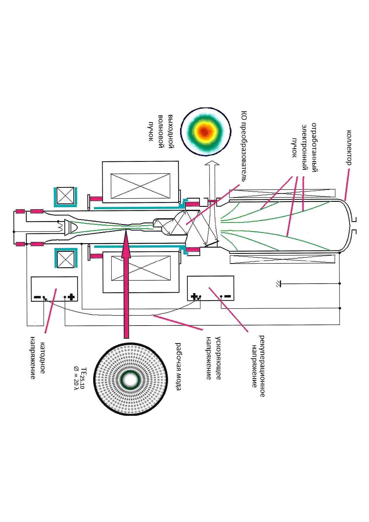
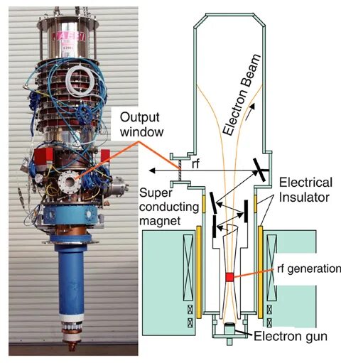
Construction references only. The first drawing shows TE₂₅,₁₀; the TRT prototype modeled here uses TE₃₃,₁₃. Their operating data are kept separate.
Fundamental harmonic; TE₃₃,₁₃ mode. Reference beam: 80 kV, 40 A, calculated pitch factor 1.2. Cavity radius 17.38 mm; beam guiding radius 7.2 mm; LaB₆ emitter diameter 86 mm. Cathode coil sensitivity: 4.56 mT/A. The JASTEC 10T150 magnet provides up to 10 T.
The supply supports up to 100 kV / 50 A. Control ranges are a teaching domain, not a guaranteed operating envelope. The displayed Ua is the anode potential relative to the grounded body. At the reference point Ua = 0 kV and the cathode is at −80 kV, so the gun-forming difference is Uak = Ua + U₀ = 80 kV. The gun solver uses Uak; changing U₀ retains the selected Ua. Both slider scales are fixed. The anode potential spans 0–20 kV and U₀ spans 20–100 kV independently, giving a forming difference Uak of 20–120 kV. All four corners of this control domain are supported. This convention applies to this laboratory only.
Generation was observed at 80 kV / 40 A over 9.13–9.29 T. Maximum output: 0.94 MW; reported efficiency: 28%, without energy recovery. The interval 9.13–9.29 T is the observed operating-mode generation range, not a constant peak-power plateau. The rounded beam parameters give P/(U₀Ib) = 29.375%, which differs from the reported 28%; no unsupported loss correction is introduced. Spectrum center: 230.1 GHz at 9.26 T. Pulses: 80 μs at 10 Hz.
A two-channel quasi-optical converter separates RF from the spent beam. High-power RF exits through a side BN vacuum window; the other channel is for an injected locking signal, which is not simulated. Electrons continue to the collector.
The anode-interception estimate uses the relativistic planar Hull criterion B_H = (mc/ed)√[(1 + eUa/mc²)² − 1]. Electrons whose local orbit reaches the anode are removed before magnetic compression and RF interaction. Ib = Ipassed + Irf + Ia. The 8 mm gap and ±8% variation are illustrative settings, not data from the TRT paper. Anode bombardment and overcurrent can precede a discharge, but do not by themselves establish a vacuum arc; gas, surface emission and plasma dynamics are not modeled.
Default Zc = 45 mm and cathode-coil contribution Bk = −0.0122 T are selected simulation settings. The paper does not report the cavity length; 45 mm is not a reconstruction of the actual tube. The axial index q = 1 is assumed. Cold-cavity frequency uses χ′₃₃,₁₃ = 83.72322656. The reference emitter field is estimated by flux conservation: Bk,total = 9.26·(7.2/43)² ≈ 0.260 T. Main-field fringe and a signed cathode-coil contribution are superposed. The drawn beam compresses continuously with r²B ≈ const; its Larmor radius follows p⊥²/B ≈ const. The axial field profile is schematic and the electron orbits are enlarged for visibility.
Without gun field maps, the same adiabatic scaling as in the first laboratory is used: q⊥ ∝ Uak²·B₀/Bk,total³ divided by squared momentum. An illustrative ±10% transverse-momentum ensemble models magnetic reflection; it is not the paper’s measured distribution. Passed electrons determine g and RF injection. The reference effective g is 1.2.
64 phases interact with a prescribed sinusoidal RF field, scanned over 0–6 MV/m. Efficiency includes reflected current; P = η·U₀·Ib is power transferred to the RF field before output losses. The displayed efficiency and power are recalculated from the selected parameters; power follows P = ηU₀Ib and is not separately fitted to 0.94 MW. Space charge, self-consistent excitation, mode competition, losses and recovery are not calculated. Searches hold Rc, Zc and their mode frequency fixed and do not prove a global maximum.